To fully understand time scale analysis, one has to understand Fourier Analysis . However, the timeseriesbook book illustrates the idea from a multivariate linear regression perspective, which is very easy to understand.

The Nyquist Frequency

The Nyquist Frequency is the highest frequency about which the data can inform us. If we have n observations, then the most number of cycles that we can observe in the time series is $n/2$.

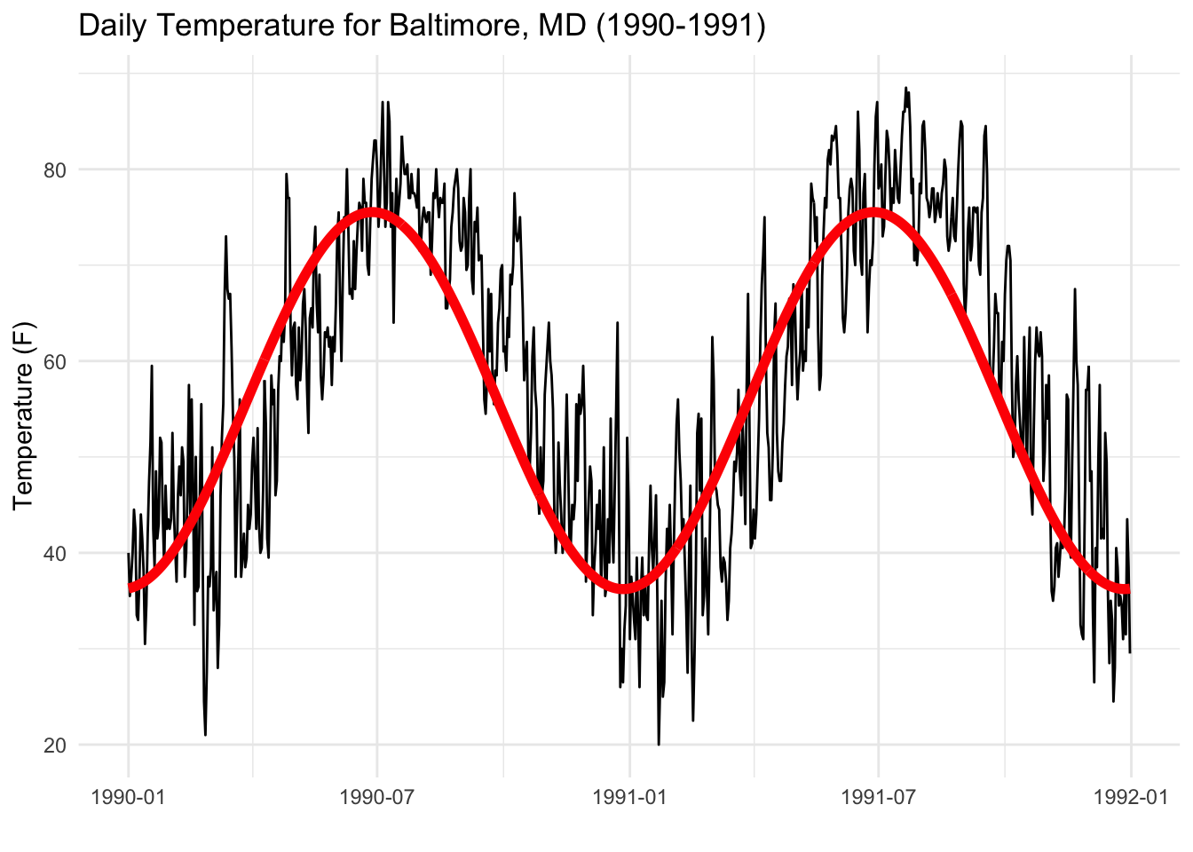
The timeseriesbook uses multivariate linear regression to introduce time scale analysis. To model the temperature of Baltimore,

we can use the following model: [ y_t = \beta_0 + \beta_1cos(2\pi t\cdot1/{365})+ \beta_2cos(2\pi t\cdot2/{365}) + \epsilon_t ]

The above model fits two cosines, one with a 1-year period and one with a half-year period. We can also fit with a 1/4 year period or 1/8 year perios. However, we cannot fit a three years period, as the observations only have two years. Also, we cannot fit half a day, as the lowest granularity of data is daily data. Thus, we can continue to add all cosines and sines terms to the model (up to n/2 of them, that is every two data points are one cycle) and see how the temperature data were correlated with each of them. The formula is:

[ y_t = a_0 + \sum_{p=1}^{n/2}\left\{ a_p \cos(2\pi tp/n)+b_p \sin(2\pi tp/n)\right\} +\epsilon_t ]

Parseval’s theorem

I like the above idea is that if the readers do not understand the Fourier Transform but understand linear regression, they can get the basic idea of this model. The timeseriesbook then illustrated how to decompose the total variation in y into the variation attributable to the various frequencies.

[ \frac1n\sum_{t=0}^{n-1}(y_t - \bar{y})^2 = \sum_{p=1}^{\frac{n}2-1}(a_p^2 + b_p^2)/2 + a_{n/2}^2 ]

Spectral Analysis

Spectral analysis is essentially to study how the energy, $R_p^2/2 =(a_p^2 + b_p^2)/2$, in each frequency range changes as a function of the frequency $p$. The plot is so-called periodogram. If we let $w_p = 2\pi p/n$, then the periodogram is:

[ I(w_p) = \frac{n}{4\pi}R_p^2 ]

The variability of the estimates of $I(w_p)$ does not go to zero as the length of the time series $n \to \infty$, as the we have more frequency coefficients to estimate when n increases. A simple way to produce a consistent estimate of $I(w_p)$ is to smooth the estimate by averaging values of $\hat{I}(w_p)$. Smoothing the periodogram needs to balance:

1. the size of the window that includes the neighboring values should increase with the sample size wot include more and more neighboring nvalues.
2. The number of points in the window relative to the total sample size should go to zero.

Well, if the above is still hard to understand, I suggest simply understand spectral analysis as a special type of ANOVA, in which each indepentent variable is those sines and cosines (frequencies), and the variation each frequency explained is the so-called energy $R_p^2/2$.

One goal of spectral analysis is to identify which indepentent variables (frequencies) have explained the most variations in the model. However, unlike the ANOVAs, the number of indepentent variables of spectral analysis will increase as the number of observations increase. Thus, smoothing windows are used to provide a consistent estimates.

The Fourier Transform

Although it is easier to understand scale analysis from the perspective of linear regresssion, I strongly suggest everyone to learn the Fourier Transform. It is so important for all engineering subjects, and it is so fun to learn. See here for more details.

The Fourier transform of a time series y t for frequency p cycles per n observations can be written as:

[ z_p = \sum_{t=0}^{n-1}y_t\mathrm{exp}(-2\pi ipt/n) ]

$z_p$ is a complex number. Its real part corresponds to the cosine variation and its imaginary part corresponds to the sine variation, based on Euler’s relation: [ \mathrm{exp}(i\theta) = \cos(\theta) + i \sin(\theta) ]

The inverse Fourier Transform is: [ y_t = \frac{1}{n}\sum_{p=0}^{n-1}z_p\mathrm{exp}(2\pi ipt/n) ]