Spatio-Temporal Statistics with R described two approaches of spatio-temporal statistical modeling. Both are trying to capture statistical dependencies in spatio-temporal phenomena, but the methods are different.

1. Descriptive modeling:

   The descriptive approach typically seeks to characterize the spatio-temporal process in terms of its mean function and its covariance function.

2. Dynamic modeling:

   The dynamic approach builds statistical models that posit (either probabilistically or mechanistically) how a spatial process changes through time.

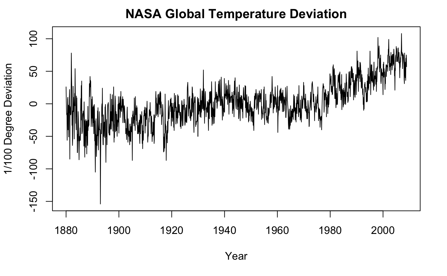
Let’s use a simple time series data to illustrate the difference between descriptive and dynamic modeling. Temperature is probably the simplest type of time series data. Here, we downloaded NASA global temperature deviation.

temp <- scan("http://stat.wharton.upenn.edu/~stine/stat910/data/nasa_global.dat")
time <- 1880 + (0:(length(temp)-1))/12
plot(time,temp, type="l", main="NASA Global Temperature Deviation", xlab="Year", \
ylab="1/100 Degree Deviation")

The dynamic approach can model the value at the current time $y_t$ as equal to a so-called “transition factor” $\phi$ times the value at the previous time $y_{t-1}$ plus and independent error $\omega_t$. [ y_t = \phi y_{t-1} +\omega_t ]

The Spatio-temporal statistics book states that

the dynamic approach is a mechanistic way of presenting the model that is easy to simulate and easy to interpret, and from a statistical perspective, dynamic models are closer to the kinds of statistical models studied in *time series.

The above model is a stationary first-order autoregressive process (AR(1)).

When we do not have a strong understanding of the mechanisms that drive the spatio-temporal phenomenon being modeled, we use the descriptive approach to study how covariates in a regssion are influencing the phenomenon.

In this case, the errors are statistically dependent in space and time. The dependence can be modeled via spatio-temporal covariances, but it can be quite difficult to specify all possible covariances for complex spatio-temporal phenomena.

In both descriptive and dynamic approaches, the models require an overwhelming computation resource, as inverting a very large covariance matrix of the data needs a lot of compuational power. To address this issue, basis functions are used to represent a spatio-temporal process as a mixed linear model. In a future blog, I will introduce more about mixed effect model and hierachical statistical model, but first we will spend a lot of time on time series analysis.

The learning curve of spatio-temporal modeling is quite steep, partly due to that it consists of both spatial modeling and time series analysis. Let’s divide and conqure. In this post and the post about the goals of spatial modeling, we mentioned about time series analysis. To understand filtering and smoothing, we have to understand state space model, which is usually introduced in time series analysis. To understand dynamic model, we have to understand time series analysis. Thus, before we dive into spatio-temporal modeling, let’s spend some time learning time series analysis.